5 Benchmarking

Below is the code used to create the fake data needed for the data processing in this document. Click to expand it! 👇

Code

library(polars)
library(arrow)
library(dplyr)
library(data.table)
library(DBI)
library(duckdb)
library(tictoc)
library(microbenchmark)
library(readr)
library(fs)
library(ggplot2)
library(pryr)
library(dbplyr)
library(forcats)
library(collapse)

# Creation the "Datasets" folder
dir.create(normalizePath("Datasets"))

set.seed(123)

# Creation of large example R data.frame
DataMultiTypes <- data.frame(
  colDate1 = as.POSIXct(sample(as.POSIXct("2023-01-01"):as.POSIXct("2023-06-30"),500000),origin="1970-01-01"),
  colDate2 = as.POSIXct(sample(as.POSIXct("2023-07-01"):as.POSIXct("2023-12-31"),500000),origin="1970-01-01"),
  colInt = sample(1:10000, 500000, replace = TRUE),
  colNum = runif(500000),
  colString = sample(c("A", "B", "C"), 500000, replace = TRUE),
  colFactor = factor(sample(c("Low", "Medium", "High"), 500000, replace = TRUE))
)

DataMultiTypes_pl <- as_polars_df(DataMultiTypes)

# Creation of large csv file
write.csv(x = DataMultiTypes,
          file = "Datasets/DataMultiTypes.csv",
          row.names=FALSE)

# Creation of unique parquet file
arrow::write_parquet(x = DataMultiTypes,
                     sink = "Datasets/DataMultiTypes.parquet")

# Creation of 6 parquet file
arrow::write_dataset(dataset = DataMultiTypes,
                     path = "Datasets/DataMultiTypes",
                     format = c("parquet"),
                     partitioning = c("colFactor"))

# Creation of duckdb file
con <- dbConnect(duckdb::duckdb(),
                 "Datasets/DataMultiTypes.duckdb")
duckdb::dbWriteTable(con,
                     "DataMultiTypes",
                     DataMultiTypes,
                     overwrite = TRUE)
dbDisconnect(con, shutdown=TRUE)

In this part of the book we will compare the performance of polars by comparing with other syntaxes, in particular R base, dplyr, dbplyr, SQL and data.table.

This section is structured according to the type of file format used for the comparison.

Note

The data processing that is performed makes very little statistical sense, but it does strive to perform some of the operations most frequently used by data scientists.

Data processing steps:

Conversion of two columns to Date format;
Filter from a integer column which must be within a range of values.
Grouping by a string column
Aggregation with calculation of the mean, minimum and maximum over two columns.

5.1 From an R object

This section analyses the different methods for making a query from an R object already loaded in memory.

Let’s start by comparing polars with R base, dplyr and data.table. We’ll alsso add collapse, a recent package that is very fast for data manipulation.

robject_polars <- function() {

  DataMultiTypes_pl$
    # Filter rows
    filter(
      pl$col("colInt")>2000 & pl$col("colInt")<8000
    )$
    # Grouping and aggregation
    group_by(
      "colString")$
    agg(
      pl$col("colInt")$min()$alias("min_colInt"),
      pl$col("colInt")$mean()$alias("mean_colInt"),
      pl$col("colInt")$max()$alias("max_colInt"),
      pl$col("colNum")$min()$alias("min_colNum"),
      pl$col("colNum")$mean()$alias("mean_colNum"),
      pl$col("colNum")$max()$alias("max_colNum")
    )
}

robject_rbase <- function() {

  # Grouping and aggregation from data filtered
  aggregate(cbind(colInt, colNum) ~ colString,
            data = DataMultiTypes[DataMultiTypes$colInt>2000 & DataMultiTypes$colInt<8000,],
            FUN = function(x) c(mean = mean(x),
                                min = min(x),
                                max = max(x)))

}

robject_dplyr <- function() {

  DataMultiTypes |>

   # Filter rows
    filter(
      colInt>2000 & colInt<8000
      ) |>

    # Grouping and aggregation
    group_by(colString) |>

    summarise(
      min_colInt = min(colInt),
      mean_colInt = mean(colInt),
      mas_colInt = max(colInt),
      min_colNum = min(colNum),
      mean_colNum = mean(colNum),
      max_colNum = max(colNum)
  )

}

robject_collapse <- function() {

  DataMultiTypes |>

   # Filter rows
    fsubset(
      colInt>2000 & colInt<8000
      ) |>

    # Grouping and aggregation
    fgroup_by(colString) |>

    fsummarise(
      min_colInt = fmin(colInt),
      mean_colInt = fmean(colInt),
      mas_colInt = fmax(colInt),
      min_colNum = fmin(colNum),
      mean_colNum = fmean(colNum),
      max_colNum = fmax(colNum)
  )

}

robject_dt <- function() {

  as.data.table(DataMultiTypes)[

    colInt > 2000 & colInt < 8000

  ][, .(min_colInt = min(colInt),
        mean_colInt = mean(colInt),
        mas_colInt = max(colInt),
        min_colNum = min(colNum),
        mean_colNum = mean(colNum),
        max_colNum = max(colNum)),

    by = colString
  ]
}

Now let’s look at how to use the DuckDb engine on R objects. There are 3 main possibilities:

To use the DuckDB engine to query a R object with dplyr, you can use the duckdb::duckdb_register() method and then the dplyr::tbl() method to pass your dplyr instructions (dplyr/DuckDB).
To use the DuckDB engine to query a R object with the standard DBI methods, you can use the duckdb::duckdb_register() method and then the DBI::dbGetQuery() method to pass your SQL query (SQL/DuckDB).
To use the DuckDB engine to query a R object in combination with {arrow} package, you can use the arrow::to_duckdb() and then pass your dplyr instructions (dplyr/arrow/DuckDB).

robject_duckdb_dplyr <- function(variables) {

  con <- DBI::dbConnect(duckdb::duckdb())

  duckdb::duckdb_register(con, "DataMultiTypes", DataMultiTypes)

  tbl(con, "DataMultiTypes") |>

    # Filter rows
    filter(
      colInt>2000 & colInt<8000
    ) |>
    # Grouping and aggregation
    group_by(colString) |>
    summarise(
      min_colInt = min(colInt, na.rm = TRUE),
      mean_colInt = mean(colInt, na.rm = TRUE),
      mas_colInt = max(colInt, na.rm = TRUE),
      min_colNum = min(colNum, na.rm = TRUE),
      mean_colNum = mean(colNum, na.rm = TRUE),
      max_colNum = max(colNum, na.rm = TRUE)
    ) |>
    collect()

  DBI::dbDisconnect(con, shutdown=TRUE)

}

robject_duckdb_sql <- function(variables) {

  con <- DBI::dbConnect(duckdb::duckdb())

  duckdb::duckdb_register(con, "DataMultiTypes", DataMultiTypes)

  DBI::dbGetQuery(
    con,
    "SELECT colString,
           MIN(colInt) AS min_colInt,
           AVG(colInt) AS mean_colInt,
           MAX(colInt) AS max_colInt,
           MIN(colNum) AS min_colNum,
           AVG(colNum) AS mean_colNum,
           MAX(colNum) AS max_colNum
    FROM (
        SELECT colString,
               colInt,
               colNum
        FROM DataMultiTypes
        WHERE colInt > 2000 AND colInt < 8000
) AS filtered_data
GROUP BY colString;")

  DBI::dbDisconnect(con, shutdown=TRUE)

}

robject_duckdb_arrow_dplyr <- function(variables) {

  DataMultiTypes |>

    to_duckdb() |>

    # Filter rows
    filter(
      colInt>2000 & colInt<8000
    ) |>
    # Grouping and aggregation
    group_by(colString) |>

    summarise(
      min_colInt = min(colInt, na.rm = TRUE),
      mean_colInt = mean(colInt, na.rm = TRUE),
      mas_colInt = max(colInt, na.rm = TRUE),
      min_colNum = min(colNum, na.rm = TRUE),
      mean_colNum = mean(colNum, na.rm = TRUE),
      max_colNum = max(colNum, na.rm = TRUE)
    )

}

Tip

One of the advantages of using the DuckDB engine and dplyr may be to use a feature implemented by DuckDB but not yet by Arrow. We can do the opposite, and return to the Arrow engine with arrow::to_arrow().

However, the benchmark results are clear: SQL queries are by far the fastest! 🏆

5.1.1 Results with a R object

microbenchmark(
  robject_polars(),
  robject_rbase(),
  robject_dplyr(),
  robject_collapse(),
  robject_dt(),
  robject_duckdb_dplyr(),
  robject_duckdb_sql(),
  robject_duckdb_arrow_dplyr(),
  times = 5
 )

Unit: milliseconds
                         expr       min        lq      mean    median        uq
             robject_polars()  12.00790  12.42099  14.43904  12.77786  14.74344
              robject_rbase() 141.70137 150.64815 184.17792 161.38329 167.22569
              robject_dplyr()  20.45172  25.84321  29.56395  32.54023  33.04592
           robject_collapse()  11.16873  11.22363  15.83778  12.42649  19.43767
                 robject_dt()  43.19118  44.38576  45.59569  44.41078  46.08512
       robject_duckdb_dplyr() 231.53580 239.20360 256.12102 241.42763 252.24654
         robject_duckdb_sql()  63.27948  63.86077  66.66307  64.67136  70.51535
 robject_duckdb_arrow_dplyr() 169.32968 169.55645 180.84764 177.02318 187.87807
       max neval
  20.24502     5
 299.93110     5
  35.93868     5
  24.93239     5
  49.90561     5
 316.19151     5
  70.98837     5
 200.45083     5

👉 Conclusion of this little benchmark using R objects already loaded in memory: the fastest to run is collapse. Next are data.table and dplyr followed closely by polars. 🏆🏆🏆 The worst performer is surprisingly duckdb with the dplyr syntax, while duckdb with the SQL language does very well and comes 4th in this ranking.

5.2 From a csv file

For this comparison, we will use :

For polars (eager), the pl$read_csv() method
For polars (lazy), the pl$scan_csv() method
For R base, the read.csv() method
For dplyr, the readr::read_csv() method
For data.table, the data.table::fread() method

csv_eager_polars <- function() {
# Reading the csv file (eager mode)
result_agg <- pl$read_csv(source = "Datasets/DataMultiTypes.csv")$
  # Conversion of 2 columns to Date format
  with_columns(
    pl$col("colDate1")$str$strptime(pl$Date, "%F %T", strict = FALSE),
    pl$col("colDate2")$str$strptime(pl$Date, "%F %T", strict = FALSE)
  )$
  # Creation of a diff column between 2 dates (in days)
  with_columns(
    (pl$col("colDate2") - pl$col("colDate1"))$dt$total_days()$alias("diff")
  )$
  # Filter rows
  filter(
    pl$col("colInt")>2000 & pl$col("colInt")<8000
  )$
  # Grouping and aggregation
  group_by(
    "colString")$
  agg(
    pl$col("colInt")$min()$alias("min_colInt"),
    pl$col("colInt")$mean()$alias("mean_colInt"),
    pl$col("colInt")$max()$alias("max_colInt"),
    pl$col("colNum")$min()$alias("min_colNum"),
    pl$col("colNum")$mean()$alias("mean_colNum"),
    pl$col("colNum")$max()$alias("max_colNum")
  )

  return(result_agg)
}
tic()
csv_eager_polars()

shape: (3, 7)
┌───────────┬────────────┬─────────────┬────────────┬────────────┬─────────────┬────────────┐
│ colString ┆ min_colInt ┆ mean_colInt ┆ max_colInt ┆ min_colNum ┆ mean_colNum ┆ max_colNum │
│ ---       ┆ ---        ┆ ---         ┆ ---        ┆ ---        ┆ ---         ┆ ---        │
│ str       ┆ i64        ┆ f64         ┆ i64        ┆ f64        ┆ f64         ┆ f64        │
╞═══════════╪════════════╪═════════════╪════════════╪════════════╪═════════════╪════════════╡
│ C         ┆ 2001       ┆ 5001.243285 ┆ 7999       ┆ 0.00003    ┆ 0.501472    ┆ 0.999992   │
│ B         ┆ 2001       ┆ 5004.31148  ┆ 7999       ┆ 0.000034   ┆ 0.500546    ┆ 0.999986   │
│ A         ┆ 2001       ┆ 4998.624945 ┆ 7999       ┆ 0.000038   ┆ 0.498445    ┆ 0.999988   │
└───────────┴────────────┴─────────────┴────────────┴────────────┴─────────────┴────────────┘

toc()

0.109 sec elapsed

csv_lazy_polars <- function() {
# Reading the csv file (eager mode)
result_agg <- pl$scan_csv(source = "Datasets/DataMultiTypes.csv")$
  # Conversion of 2 columns to Date format
  with_columns(
    pl$col("colDate1")$str$strptime(pl$Date, "%F %T", strict = FALSE),
    pl$col("colDate2")$str$strptime(pl$Date, "%F %T", strict = FALSE)
  )$
  # Creation of a diff column between 2 dates (in days)
  with_columns(
    (pl$col("colDate2") - pl$col("colDate1"))$dt$total_days()$alias("diff")
  )$
  # Filter rows
  filter(
    pl$col("colInt")>2000 & pl$col("colInt")<8000
  )$
  # Grouping and aggregation
  group_by(
    "colString")$
  agg(
    pl$col("colInt")$min()$alias("min_colInt"),
    pl$col("colInt")$mean()$alias("mean_colInt"),
    pl$col("colInt")$max()$alias("max_colInt"),
    pl$col("colNum")$min()$alias("min_colNum"),
    pl$col("colNum")$mean()$alias("mean_colNum"),
    pl$col("colNum")$max()$alias("max_colNum")
  )

  return(result_agg)
}
tic()
csv_lazy_polars()$collect()

shape: (3, 7)
┌───────────┬────────────┬─────────────┬────────────┬────────────┬─────────────┬────────────┐
│ colString ┆ min_colInt ┆ mean_colInt ┆ max_colInt ┆ min_colNum ┆ mean_colNum ┆ max_colNum │
│ ---       ┆ ---        ┆ ---         ┆ ---        ┆ ---        ┆ ---         ┆ ---        │
│ str       ┆ i64        ┆ f64         ┆ i64        ┆ f64        ┆ f64         ┆ f64        │
╞═══════════╪════════════╪═════════════╪════════════╪════════════╪═════════════╪════════════╡
│ B         ┆ 2001       ┆ 5004.31148  ┆ 7999       ┆ 0.000034   ┆ 0.500546    ┆ 0.999986   │
│ A         ┆ 2001       ┆ 4998.624945 ┆ 7999       ┆ 0.000038   ┆ 0.498445    ┆ 0.999988   │
│ C         ┆ 2001       ┆ 5001.243285 ┆ 7999       ┆ 0.00003    ┆ 0.501472    ┆ 0.999992   │
└───────────┴────────────┴─────────────┴────────────┴────────────┴─────────────┴────────────┘

toc()

0.046 sec elapsed

csv_rbase <- function() {

  # Reading the csv file
  result <- read.csv("Datasets/DataMultiTypes.csv")

  # Conversion of 2 columns to Date format
  result$colDate1 <- as.Date(result$colDate1)
  result$colDate2 <- as.Date(result$colDate2)

  # Creation of a diff column between 2 dates (in days)
  result$diff <- round(
    as.integer(
      difftime(
        result$colDate2,
        result$colDate1,
        units = "days")
      ),
    0)

  # Filter rows
  result <- result[result$colInt>2000 & result$colInt<8000,]

  # Grouping and aggregation
  result_agg <- aggregate(cbind(colInt, colNum) ~ colString,
                          data = result,
                          FUN = function(x) c(mean = mean(x),
                                              min = min(x),
                                              max = max(x)))

  return(result_agg)
}

tic()
res_rbase <- csv_rbase()
toc()

6.536 sec elapsed

print(res_rbase)

  colString colInt.mean colInt.min colInt.max  colNum.mean   colNum.min
1         A    4998.625   2001.000   7999.000 4.984446e-01 3.794138e-05
2         B    5004.311   2001.000   7999.000 5.005457e-01 3.385660e-05
3         C    5001.243   2001.000   7999.000 5.014723e-01 3.045052e-05
    colNum.max
1 9.999879e-01
2 9.999863e-01
3 9.999921e-01

csv_dplyr <- function() {

  # Reading the csv file
  result <- readr::read_csv("Datasets/DataMultiTypes.csv", show_col_types = FALSE)

  # Conversion of 2 columns to Date format
  result <- result |>
    mutate(
      colDate1 = as.Date(colDate1),
      colDate2 = as.Date(colDate2)
    )

  # Creation of a diff column between 2 dates (in days)
  result <- result |>
    mutate(diff = round(as.integer(difftime(colDate2, colDate1, units = "days")),0))

  # Filter rows
  result <- result |>
    filter(
      colInt>2000 & colInt<8000
      )

  # Grouping and aggregation
  result_agg <- result |>
    group_by(colString) |>
    summarise(
      min_colInt = min(colInt),
      mean_colInt = mean(colInt),
      mas_colInt = max(colInt),
      min_colNum = min(colNum),
      mean_colNum = mean(colNum),
      max_colNum = max(colNum)
  )

  return(result_agg)
}

tic()
res_dplyr <- csv_dplyr()
toc()

0.39 sec elapsed

print(res_dplyr)

# A tibble: 3 × 7
  colString min_colInt mean_colInt mas_colInt min_colNum mean_colNum max_colNum
  <chr>          <dbl>       <dbl>      <dbl>      <dbl>       <dbl>      <dbl>
1 A               2001       4999.       7999  0.0000379       0.498      1.000
2 B               2001       5004.       7999  0.0000339       0.501      1.000
3 C               2001       5001.       7999  0.0000305       0.501      1.000

csv_arrow <- function() {

  # Reading the csv file
  result <- arrow::read_csv_arrow("Datasets/DataMultiTypes.csv", as_data_frame = FALSE)

  # Conversion of 2 columns to Date format
  result <- result |>
    mutate(
      colDate1 = as.Date(colDate1),
      colDate2 = as.Date(colDate2)
    )

  # Creation of a diff column between 2 dates (in days)
  result <- result |>
    # difftime(unit = "days") is not supported in arrow yet
    mutate(diff = round(as.integer64(difftime(colDate2, colDate1)) %/% (60 * 60 * 24), 0))

  # Filter rows
  result <- result |>
    filter(
      colInt>2000 & colInt<8000
      )

  # Grouping and aggregation
  result_agg <- result |>
    group_by(colString) |>
    summarise(
      min_colInt = min(colInt),
      mean_colInt = mean(colInt),
      mas_colInt = max(colInt),
      min_colNum = min(colNum),
      mean_colNum = mean(colNum),
      max_colNum = max(colNum)
  ) |>
    collect()

  return(result_agg)
}

tic()
res_arrow <- csv_arrow()
toc()

0.244 sec elapsed

print(res_arrow)

# A tibble: 3 × 7
  colString min_colInt mean_colInt mas_colInt min_colNum mean_colNum max_colNum
  <chr>          <int>       <dbl>      <int>      <dbl>       <dbl>      <dbl>
1 B               2001       5004.       7999  0.0000339       0.501      1.000
2 C               2001       5001.       7999  0.0000305       0.501      1.000
3 A               2001       4999.       7999  0.0000379       0.498      1.000

csv_dt <- function() {

  result_agg <- as.data.table(data.table::fread("Datasets/DataMultiTypes.csv"))[, `:=`(

  colDate1 = as.Date(colDate1),
  colDate2 = as.Date(colDate2),
  diff = as.integer(difftime(colDate2, colDate1, units = "days"))

)][colInt > 2000 & colInt < 8000, .(

  min_colInt = min(colInt),
  mean_colInt = mean(colInt),
  max_colInt = max(colInt),
  min_colNum = min(colNum),
  mean_colNum = mean(colNum),
  max_colNum = max(colNum)

), by = colString]

  return(result_agg)
}
tic()
csv_dt()

   colString min_colInt mean_colInt max_colInt   min_colNum mean_colNum
      <char>      <int>       <num>      <int>        <num>       <num>
1:         B       2001    5004.311       7999 3.385660e-05   0.5005457
2:         C       2001    5001.243       7999 3.045052e-05   0.5014723
3:         A       2001    4998.625       7999 3.794138e-05   0.4984446
   max_colNum
        <num>
1:  0.9999863
2:  0.9999921
3:  0.9999879

toc()

0.178 sec elapsed

Note

The data processing performed is not entirely equivalent, since it includes in addition: - for polars (lazy mode), conversion to data.frame R at the end of processing - for data.table, conversion to dt format at the start, then conversion to data.frame R at the end of processing

5.2.1 Results eager vs lazy mode

csv_bmk <- microbenchmark(
  "polars (eager) from csv file" = csv_eager_polars(),
  "polars (lazy) from csv file" = csv_lazy_polars()$collect(),
  "R base - from csv file" = csv_rbase(),
  "dplyr - from csv file" = csv_dplyr(),
  "dplyr (Acero) - from csv file" = csv_arrow(),
  "data.table - from csv file" = csv_dt(),
  times = 5
 )
csv_bmk

Unit: milliseconds
                          expr       min         lq       mean    median
  polars (eager) from csv file  100.4107  104.44400  107.22650  105.5091
   polars (lazy) from csv file   41.5927   41.73844   44.78536   42.2385
        R base - from csv file 5539.4923 5568.00176 5648.44625 5634.6846
         dplyr - from csv file  315.8509  324.93070  429.37978  480.7258
 dplyr (Acero) - from csv file  154.2273  156.41234  162.33605  157.1189
    data.table - from csv file  106.2667  122.96019  204.51577  132.7937
         uq        max neval
  105.54307  120.22562     5
   42.31532   56.04185     5
 5705.71878 5794.33380     5
  486.39342  538.99816     5
  158.99038  184.93128     5
  287.70828  372.84998     5

👉 Conclusion of this little benchmark based on csv files: the big winners are polars (eager mode) and dplyr with {arrow}. The results will undoubtedly be even better with polars (lazy mode)… 🏆🏆🏆 TO DO !!!

5.3 From an unique parquet file

For this comparison on unique parquet file, we will use :

For polars (lazy), the pl$scan_parquet() method
For arrow (eager), the arrow::read_parquet() method
For arrow (lazy), the arrow::open_dataset() method
For Duckdb and SQL, the arrow::read_parquet() and DBI::dbGetQuery() methods

Note

With arrow, you can use the following verbs from the tidyverse to do transformations on your tables.

parquet_polars_lazy <- function(variables) {

  result <- pl$scan_parquet(source = "Datasets/DataMultiTypes.parquet")$
    # Conversion of 2 columns to Date format
    with_columns(
      pl$col("colDate1")$str$strptime(pl$Date, "%F %T", strict = FALSE),
      pl$col("colDate2")$str$strptime(pl$Date, "%F %T", strict = FALSE)
    )$
    # Filter rows
    filter(
      pl$col("colInt")>2000 & pl$col("colInt")<8000
    )$
    # Grouping and aggregation
    group_by(
      "colString")$
    agg(
      pl$col("colInt")$min()$alias("min_colInt"),
      pl$col("colInt")$mean()$alias("mean_colInt"),
      pl$col("colInt")$max()$alias("max_colInt"),
      pl$col("colNum")$min()$alias("min_colNum"),
      pl$col("colNum")$mean()$alias("mean_colNum"),
      pl$col("colNum")$max()$alias("max_colNum")
    )

  return(result)
}
tic()
as.data.frame(parquet_polars_lazy()$collect())

  colString min_colInt mean_colInt max_colInt   min_colNum mean_colNum
1         A       2001    4998.625       7999 3.794138e-05   0.4984446
2         B       2001    5004.311       7999 3.385660e-05   0.5005457
3         C       2001    5001.243       7999 3.045052e-05   0.5014723
  max_colNum
1  0.9999879
2  0.9999863
3  0.9999921

toc()

0.029 sec elapsed

arrow_eager <- function(variables) {

  result <- arrow::read_parquet("Datasets/DataMultiTypes.parquet") |>

    mutate(
      # Conversion of 2 columns to Date format
      colDate1 = as.Date(colDate1),
      colDate2 = as.Date(colDate2)
    ) |>
    # Filter rows
    filter(
      colInt>2000 & colInt<8000
    ) |>
    # Grouping and aggregation
    group_by(colString) |>
    summarise(
      min_colInt = min(colInt),
      mean_colInt = mean(colInt),
      mas_colInt = max(colInt),
      min_colNum = min(colNum),
      mean_colNum = mean(colNum),
      max_colNum = max(colNum)
  )

  return(result)

}
tic()
arrow_eager()

# A tibble: 3 × 7
  colString min_colInt mean_colInt mas_colInt min_colNum mean_colNum max_colNum
  <chr>          <int>       <dbl>      <int>      <dbl>       <dbl>      <dbl>
1 A               2001       4999.       7999  0.0000379       0.498      1.000
2 B               2001       5004.       7999  0.0000339       0.501      1.000
3 C               2001       5001.       7999  0.0000305       0.501      1.000

toc()

0.099 sec elapsed

arrow_lazy <- function(variables) {

  result <- arrow::open_dataset("Datasets/DataMultiTypes.parquet") |>

    mutate(
      # Conversion of 2 columns to Date format
      colDate1 = as.Date(colDate1),
      colDate2 = as.Date(colDate2)
    ) |>
    # Filter rows
    filter(
      colInt>2000 & colInt<8000
    ) |>
    # Grouping and aggregation
    group_by(colString) |>
    summarise(
      min_colInt = min(colInt),
      mean_colInt = mean(colInt),
      mas_colInt = max(colInt),
      min_colNum = min(colNum),
      mean_colNum = mean(colNum),
      max_colNum = max(colNum)
  )

  return(result)

}
tic()
arrow_lazy() |> collect()

# A tibble: 3 × 7
  colString min_colInt mean_colInt mas_colInt min_colNum mean_colNum max_colNum
  <chr>          <int>       <dbl>      <int>      <dbl>       <dbl>      <dbl>
1 B               2001       5004.       7999  0.0000339       0.501      1.000
2 A               2001       4999.       7999  0.0000379       0.498      1.000
3 C               2001       5001.       7999  0.0000305       0.501      1.000

toc()

0.141 sec elapsed

parquet_duckdb_sql <- function(variables) {

  con <- dbConnect(duckdb::duckdb())

  result <- dbGetQuery(
    con,
    "SELECT colString,
           MIN(colInt) AS min_colInt,
           AVG(colInt) AS mean_colInt,
           MAX(colInt) AS max_colInt,
           MIN(colNum) AS min_colNum,
           AVG(colNum) AS mean_colNum,
           MAX(colNum) AS max_colNum
    FROM (
        SELECT colString,
               colInt,
               colNum
        FROM read_parquet('Datasets/DataMultiTypes.parquet')
        WHERE colInt > 2000 AND colInt < 8000
) AS filtered_data
GROUP BY colString;")

  dbDisconnect(con, shutdown=TRUE)

  return(result)
}
tic()
parquet_duckdb_sql()

  colString min_colInt mean_colInt max_colInt   min_colNum mean_colNum
1         C       2001    5001.243       7999 3.045052e-05   0.5014723
2         B       2001    5004.311       7999 3.385660e-05   0.5005457
3         A       2001    4998.625       7999 3.794138e-05   0.4984446
  max_colNum
1  0.9999921
2  0.9999863
3  0.9999879

toc()

0.071 sec elapsed

5.3.1 Results for unique parquet file

unique_parquet_bmk <- microbenchmark(
  "polars (lazy) - from unique parquet file" = as.data.frame(parquet_polars_lazy()$collect()),
  "arrow (eager) - from unique parquet file" = arrow_eager(),
  "arrow (lazy) - from unique parquet file" = arrow_lazy() |> collect(),
  "Duckdb and SQL - from unique parquet file" = parquet_duckdb_sql(),
  times = 5
 )
print(unique_parquet_bmk)

Unit: milliseconds
                                      expr       min        lq      mean
  polars (lazy) - from unique parquet file  19.40738  20.36978  23.45683
  arrow (eager) - from unique parquet file  73.88778  86.62267  85.64054
   arrow (lazy) - from unique parquet file 110.94717 111.81999 119.16319
 Duckdb and SQL - from unique parquet file  47.65263  48.94167  51.68237
    median        uq       max neval
  20.94607  21.11533  35.44560     5
  87.74994  88.78745  91.15486     5
 119.47904 119.77565 133.79412     5
  51.15989  54.76752  55.89016     5

👉 Conclusion of this little benchmark based on unique parquet files: the big winner is polars (lazy mode) ! 🏆🏆🏆

5.4 From a partitioned parquet file

Let’s now look at how to perform queries on partitioned files.

The structure of partitioned files on the disk is as follows:

fs::dir_tree(path = "Datasets/DataMultiTypes/")

Datasets/DataMultiTypes/
├── colFactor=High
│   └── part-0.parquet
├── colFactor=Low
│   └── part-0.parquet
└── colFactor=Medium
    └── part-0.parquet

For this comparison, we will use :

For arrow (lazy), the arrow::open_dataset() method
For dplyr (duckdb), the DBI::dbConnect, dplyr::tbl() and arrow::read_parquet() methods
For polars (lazy), the pl$scan_parquet() method

partitioned_parquet_arrow_lazy <- function(variables) {

  result <- arrow::open_dataset(
    "Datasets/DataMultiTypes/",
    partitioning = arrow::schema(colFactor = arrow::utf8())) |>

    mutate(
      # Conversion of 2 columns to Date format
      colDate1 = as.Date(colDate1),
      colDate2 = as.Date(colDate2)
    ) |>
    # Filter rows
    filter(
      colInt>2000 & colInt<8000
    ) |>
    # Grouping and aggregation
    group_by(colString) |>
    summarise(
      min_colInt = min(colInt),
      mean_colInt = mean(colInt),
      mas_colInt = max(colInt),
      min_colNum = min(colNum),
      mean_colNum = mean(colNum),
      max_colNum = max(colNum)
    ) |>
    collect()

  return(result)

}
tic()
partitioned_parquet_arrow_lazy()

# A tibble: 3 × 7
  colString min_colInt mean_colInt mas_colInt min_colNum mean_colNum max_colNum
  <chr>          <int>       <dbl>      <int>      <dbl>       <dbl>      <dbl>
1 B               2001       5004.       7999  0.0000339       0.501      1.000
2 C               2001       5001.       7999  0.0000305       0.501      1.000
3 A               2001       4999.       7999  0.0000379       0.498      1.000

toc()

0.133 sec elapsed

# library(dbplyr)

partitioned_parquet_dplyr_duckdb <- function(variables) {

  con <- DBI::dbConnect(duckdb::duckdb())

  result <- tbl(con, "read_parquet('Datasets/DataMultiTypes/*/*.parquet', hive_partitioning=1)") |>

    mutate(
      # Conversion of 2 columns to Date format
      colDate1 = as.Date(colDate1),
      colDate2 = as.Date(colDate2)
    ) |>
    # Filter rows
    filter(
      colInt>2000 & colInt<8000
    ) |>
    # Grouping and aggregation
    group_by(colString) |>
    summarise(
      min_colInt = min(colInt, na.rm = TRUE),
      mean_colInt = mean(colInt, na.rm = TRUE),
      mas_colInt = max(colInt, na.rm = TRUE),
      min_colNum = min(colNum, na.rm = TRUE),
      mean_colNum = mean(colNum, na.rm = TRUE),
      max_colNum = max(colNum, na.rm = TRUE)
    ) |>
    collect()

  DBI::dbDisconnect(con)
  return(result)
}
tic()
partitioned_parquet_dplyr_duckdb()

# A tibble: 3 × 7
  colString min_colInt mean_colInt mas_colInt min_colNum mean_colNum max_colNum
  <chr>          <int>       <dbl>      <int>      <dbl>       <dbl>      <dbl>
1 B               2001       5004.       7999  0.0000339       0.501      1.000
2 A               2001       4999.       7999  0.0000379       0.498      1.000
3 C               2001       5001.       7999  0.0000305       0.501      1.000

toc()

0.317 sec elapsed

partitioned_parquet_polars_lazy <- function(variables) {

  result <- pl$scan_parquet(source = "Datasets/DataMultiTypes.parquet")$
    # Conversion of 2 columns to Date format
    with_columns(
      pl$col("colDate1")$str$strptime(pl$Date, "%F %T", strict = FALSE),
      pl$col("colDate2")$str$strptime(pl$Date, "%F %T", strict = FALSE)
    )$
    # Filter rows
    filter(
      pl$col("colInt")>2000 & pl$col("colInt")<8000
    )$
    # Grouping and aggregation
    group_by(
      "colString")$
    agg(
      pl$col("colInt")$min()$alias("min_colInt"),
      pl$col("colInt")$mean()$alias("mean_colInt"),
      pl$col("colInt")$max()$alias("max_colInt"),
      pl$col("colNum")$min()$alias("min_colNum"),
      pl$col("colNum")$mean()$alias("mean_colNum"),
      pl$col("colNum")$max()$alias("max_colNum")
    )$collect()

  return(result)
}
tic()
partitioned_parquet_polars_lazy()

shape: (3, 7)
┌───────────┬────────────┬─────────────┬────────────┬────────────┬─────────────┬────────────┐
│ colString ┆ min_colInt ┆ mean_colInt ┆ max_colInt ┆ min_colNum ┆ mean_colNum ┆ max_colNum │
│ ---       ┆ ---        ┆ ---         ┆ ---        ┆ ---        ┆ ---         ┆ ---        │
│ str       ┆ i32        ┆ f64         ┆ i32        ┆ f64        ┆ f64         ┆ f64        │
╞═══════════╪════════════╪═════════════╪════════════╪════════════╪═════════════╪════════════╡
│ A         ┆ 2001       ┆ 4998.624945 ┆ 7999       ┆ 0.000038   ┆ 0.498445    ┆ 0.999988   │
│ B         ┆ 2001       ┆ 5004.31148  ┆ 7999       ┆ 0.000034   ┆ 0.500546    ┆ 0.999986   │
│ C         ┆ 2001       ┆ 5001.243285 ┆ 7999       ┆ 0.00003    ┆ 0.501472    ┆ 0.999992   │
└───────────┴────────────┴─────────────┴────────────┴────────────┴─────────────┴────────────┘

toc()

0.021 sec elapsed

5.4.1 Results for partitioned parquet files

partitioned_parquet_bmk <- microbenchmark(
  "arrow (lazy) - from partitioned parquet file" = partitioned_parquet_arrow_lazy(),
  "dplyr (duckdb) - from partitioned parquet file" = partitioned_parquet_dplyr_duckdb(),
  "polars (lazy) - from partitioned parquet file" = as.data.frame(partitioned_parquet_polars_lazy()),
  times = 5
 )
print(partitioned_parquet_bmk)

Unit: milliseconds
                                           expr       min        lq      mean
   arrow (lazy) - from partitioned parquet file 108.59320 108.75808 112.21279
 dplyr (duckdb) - from partitioned parquet file 254.13925 260.15026 287.42754
  polars (lazy) - from partitioned parquet file  18.47431  18.75874  21.26151
    median        uq       max neval
 108.88159 116.96340 117.86767     5
 266.29269 313.58977 342.96574     5
  19.21465  19.63563  30.22422     5

👉 Conclusion of this little benchmark based on partitioned parquet files: as for unique parquet files, the big winner is polars (lazy mode) ! 🏆🏆🏆

5.5 From a DuckDb file

Let’s look at how to perform queries on duckdb files.

For this comparison, we will use :

For SQL, the DBI::dbGetQuery() method. In this way, we use the standard DBI methods to work from a DuckDb file.

duckdb_dbfile_sql <- function(variables) {
  
  con <- dbConnect(duckdb::duckdb(),
                 "Datasets/DataMultiTypes.duckdb")
  
  result <- dbGetQuery(
    con, 
    "SELECT colString,
           MIN(colInt) AS min_colInt,
           AVG(colInt) AS mean_colInt,
           MAX(colInt) AS max_colInt,
           MIN(colNum) AS min_colNum,
           AVG(colNum) AS mean_colNum,
           MAX(colNum) AS max_colNum
    FROM (
        SELECT colString,
               colInt,
               colNum
        FROM DataMultiTypes
        WHERE colInt > 2000 AND colInt < 8000
) AS filtered_data
GROUP BY colString;")
  
  dbDisconnect(con, shutdown=TRUE)
  
  return(result)
  
}
tic()
duckdb_dbfile_sql()

  colString min_colInt mean_colInt max_colInt   min_colNum mean_colNum
1         A       2001    4998.625       7999 3.794138e-05   0.4984446
2         B       2001    5004.311       7999 3.385660e-05   0.5005457
3         C       2001    5001.243       7999 3.045052e-05   0.5014723
  max_colNum
1  0.9999879
2  0.9999863
3  0.9999921

toc()

0.056 sec elapsed

5.5.1 Results for DuckDB file

duckdb_bmk <- microbenchmark(
  "SQL from duckdb file" = duckdb_dbfile_sql(),
  times = 5
 )
duckdb_bmk

Unit: milliseconds
                 expr      min       lq     mean   median       uq    max neval
 SQL from duckdb file 48.26395 48.31936 50.46011 49.78774 50.42653 55.503     5

Note that the query with the standard DBI methods is faster than those with dplyr verbs 🏆

5.6 Final results

5.6.1 Performance

So what can we conclude?
With which file format and which method is it fastest to execute the same request?

Let’s have a look! First, let’s aggregate all the benchmark results:

# Aggregation
bmk_results <- rbind(
  csv_bmk,
  unique_parquet_bmk,
  partitioned_parquet_bmk,
  duckdb_bmk
)

Let’s do a quick sort on the expr column before plotting the results :

Code

# Sort the results
bmk_results$expr <- reorder(bmk_results$expr, bmk_results$time, decreasing = TRUE)

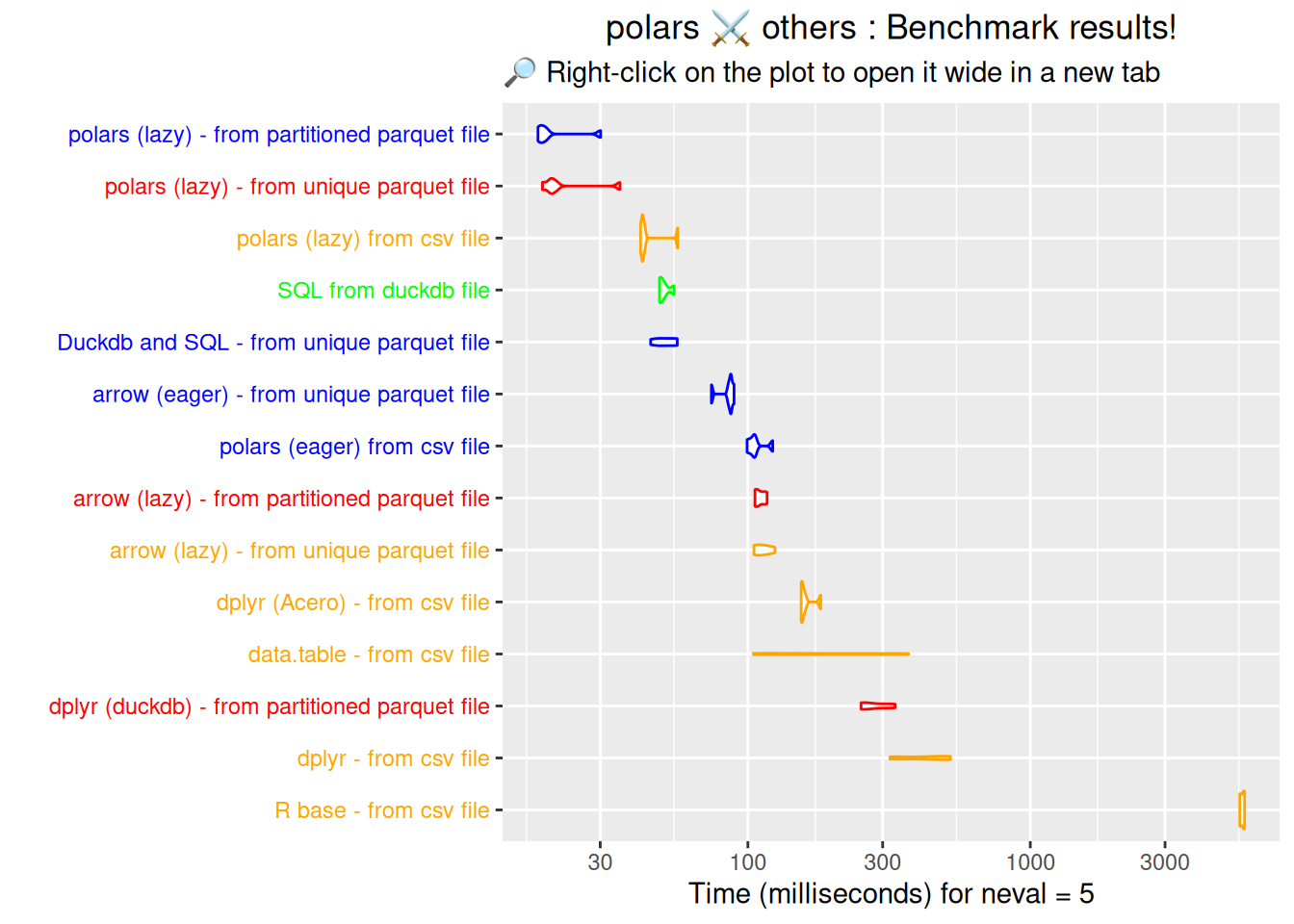
Final conclusions

👉 A few conclusions can be drawn from this section on benchmarking:

It is more efficient to work from a parquet or duckdb file except for polars with lazy evaluation which is very fast;
In terms of execution speed, there is no great difference between a single parquet file and several partitioned parquet files (although the gap will undoubtedly widen in favour of partitioned files if the size of the initial work file is increased);
Lazy evaluation of polars performs best whatever the format of the file you are working on. 🏆🏆
It’s followed by SQL queries executed directly on a duckdb file. 🏆

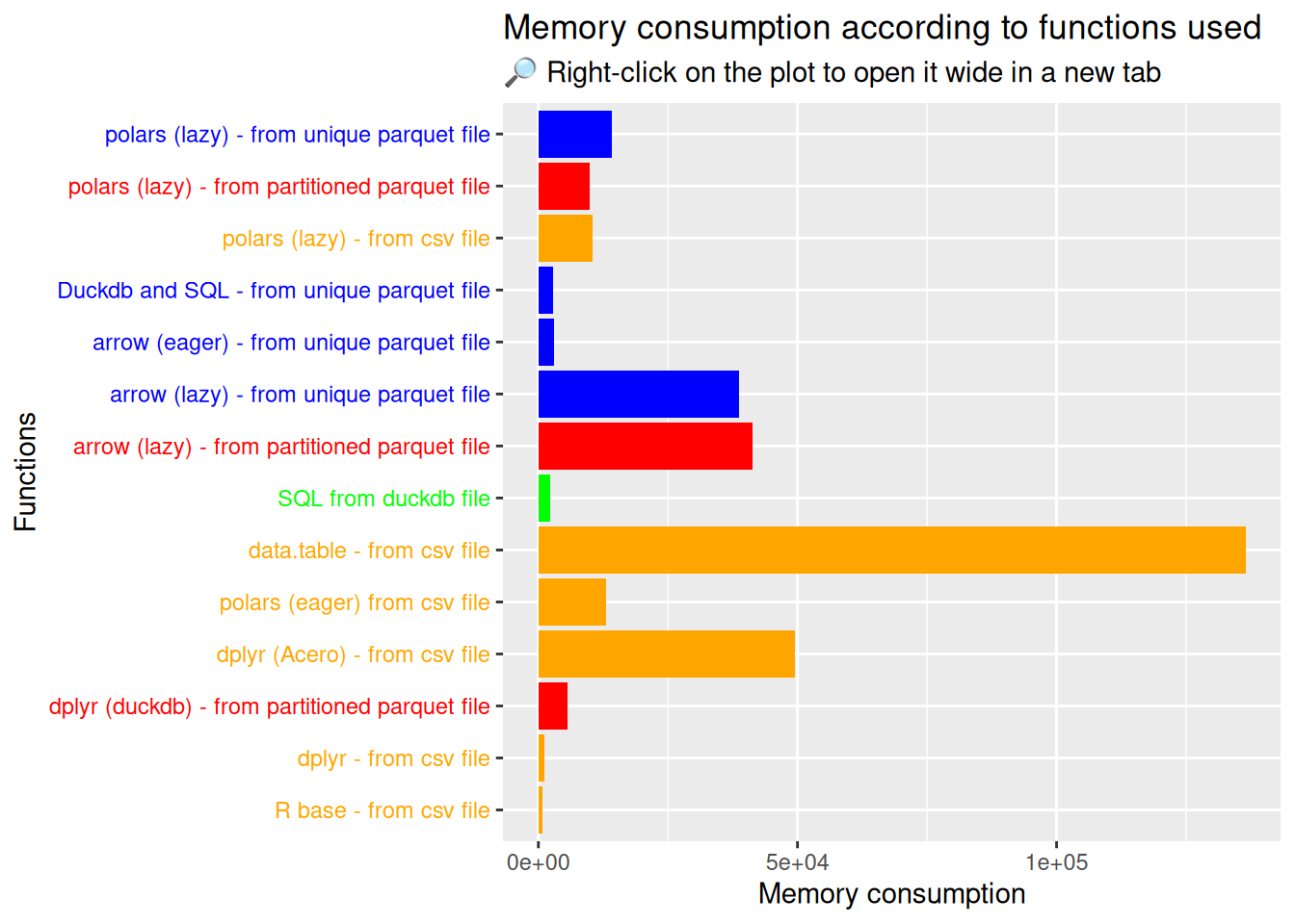
5.6.2 Memory usage

We’ve just analysed the performance of the various alternatives to Polars, but what about R’s memory usage?

To do this, we’re going to use mem_change() from {pryr} package. This method tells you how memory changes during code execution. Positive numbers represent an increase in the memory used by R, and negative numbers represent a decrease.

Memory usage conclusions

👉 A few conclusions can be drawn from this section on benchmarking about memory usage:

Firstly, the method with data.table from a csv file surprisingly consumes a lot of RAM. Maybe it’s related to the as.data.table() conversion? If a reader has an explanation, I’m interested and feel free to open an issue;
Regarding csv files, syntaxes with R base and dplyr are the least consuming RAM (but at the expense of speed);
Regarding parquet files, syntaxes with arrow (eager) and Duckdb with SQL are the least consuming RAM;
The SQL language used on a Duckdb file also consumes very little RAM

🏆🏆🏆